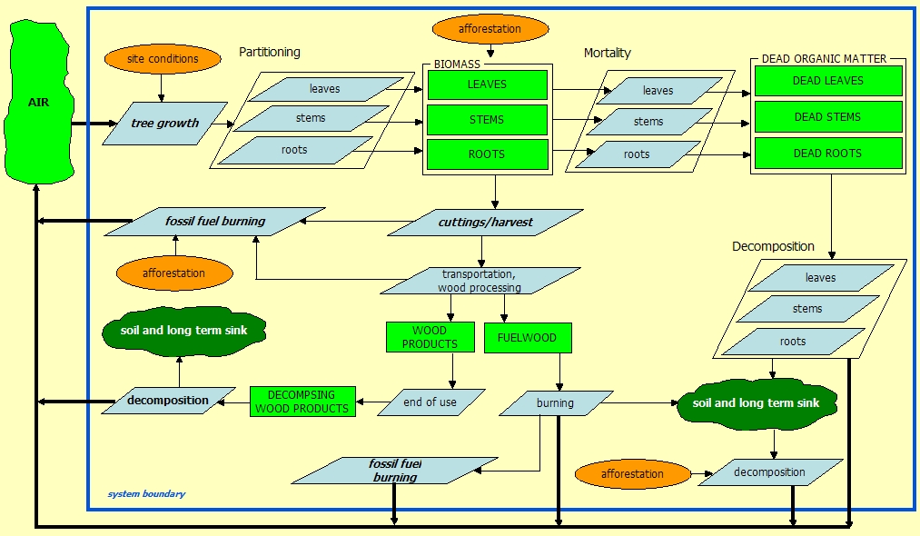
Processes are fluxes that change the size (i.e. content) of the pools. They are denoted by blue diamonds on the flowchart.

Growth is the process of increasing plant biomass through net photosynthesis, the prosess in which carbon dioxide of the air is fixed by leaves, in form of various types of organic matter, by using the energy of the sunlight. Net photosynthesis is gross photosynthesis minus respiration: in order for live plants to function, they must use some parts of the organic matter produced to get energy from. This process is called respiration. The change of biomass is therefore a net change, i.e. the difference between (gross) assimilation and respiration. Under some circumstances, respiration can be higher than gross assimilation, but normally the latter is bigger.

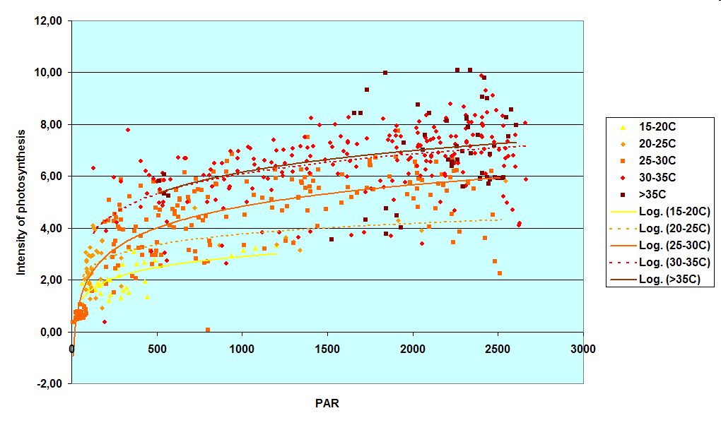
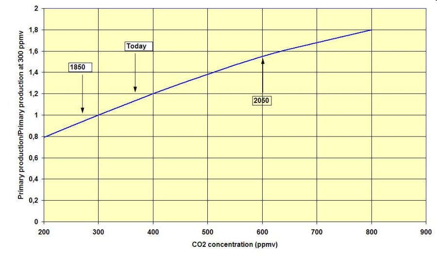
All these processes depend on environmental variables like light and temperature (see graph on photosynthetic activity over light intensity and temperature as an example). The CO₂ concentration of the air also affects photosynthesis (see graph), however, the long-term effects are poorly understood yet.

Photosynthesis and respiraton are not directly modelled here. In order to do that, continuous measurements of environmental conditions (light, temperature, humidity, precipitation etc.) would be required, which is theoretically impossible for predictions. Rather, net primary production (NPP) is estimated by using growth models, in which historical growth trends are taken as long-term average of past periods. These models are known as yield models, and they have been used in forestry practice for centuries. (Quite naturally, these models were repeatedly developed and improved, incorporating new measurements and other knowledge on tree and stand growth.)

However, yield models only contain data for above ground tree volume, therefore, in estimating above ground assimilation rate expressed as ton carbon per year (or current net primary carbon production, CPCP), estimating aboveground tree volume increment is only the first of five steps to obtain total biomass production. In the second step, the volume increment is multiplied by a biomass expansion factor (BEF, see below), to get aboveground woody biomass increment. In the third steps, factors are used to convert biomass values to carbon values (see below):

CGWPCP for the whole forest area can be calculated by multiplying CGWPCP by the area of forest land.

In the fourth step, the increment of other biomass components (i.e. leaves and roots) is calculated by using BEFs from CGWPCP, and finally, all biomass increments are totalled to arrive at NPP (expressed in amount of carbon; see also the biomass section).

Note that "net" and "gross" is used in various ways. "Net" primary production is the difference between the rate of photosynthesis and respiration, but it is also a "gross" value ("gross" increment), because "net" increment is the difference of "gross" increment and mortality.

Baseline scenario: at this stage of model development it is supposed that the change of the carbon content of the system is zero.

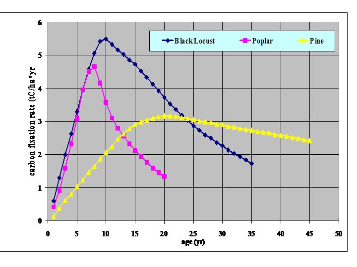
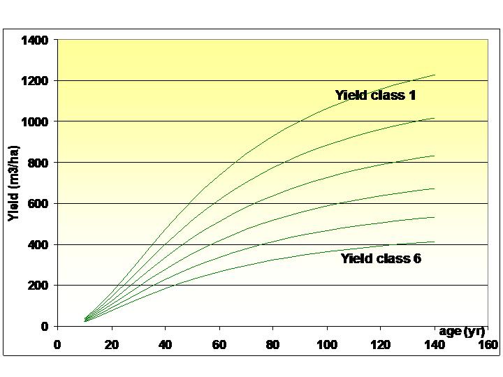
CAI on unit land is usually estimated by using yield models. Forest yield models provide growth data for unit land by species, age and yield class. (Most yield models are for unmixed stands; mixed stands are usually taken as the sum of two distinct pure substands.) A graphical example is given here for one yield class by species and age, and another for one species by age and yield class.

CASMOFOR uses standard yield tables for the most important tree species in Hungary. These models were developed by the Hungarian Forest Research Institute, and are in general use in the country. Of the various versions of the yield models, the lates versions are used in CASMOFOR. These yield tables are the following (see also credits):

Species	Year of publication	Author(s)
Black locust	1984	Rédei K.
Beech	1983	Mendlik G
Turkey oak	1983	Kovács F.
Scotch pine	1992	Solymos R.
Silver linden	1995	Hajdu G.
Black walnut	1973	Palotás F.
Black pine	1992	Kovács F., Veperdi G.
White poplar	1992	Rédei K.
White willow	1969	Palotás F.
Hornbeam	1983	Béky A.
Hornbeam-Sessile oak	1995	Béky A., Somogyi Z.
Pedunculate oak	1988	Kiss R., Somogyi Z., Juhász Gy.
Sessile oak, seed	1981	Béky A.
Sessile oak, coppice	1989	Béky A.
Norway spruce	1973	Solymos R.
Common alder	1972	Adorján J.
Common ash	1988	Kovács F.
Betula	1981	Rumszauer J.
Hybrid poplar	1980	Halupa L.
Larch	1974	Tuskó L.
Red oak	1991	Rédei K.

Béky, A. 1981. Mag eredetű kocsánytalan tölgyesek fatermése. Erdészeti Kutatások 74:309-320.

Béky, A. 1983. Országos fatermési tábla gyertyán állományokra. Erdészeti Kutatások 75:199-208.

Béky, A. 1991. Ertrag von Traubeneichen-Niederwälder. Erdészeti Kutatások 82-83:176-192.

Béky, A. 1991. Sarj kocsánytalan tölgyek fatermése. Erdészeti Kutatások 82-83/II:181-197.

Béky, A., Somogyi, Z. 1995. Fatermési tábla optimális szerkezetű gyertyános-kocsánytalan tölgyesekre. Erdészeti Kutatások 85:49-78.

Bondor, A. 1984. A szelídgesztenye fatermése. Erdészeti Kutatások 76-77:133-150.

Hajdu, G. 1995. Ezüsthárs (Tilia tomentosa Mönch.) fatermési táblázatok. Erdészeti Kutatások 85:113-124.

Halupa, L., Kiss, R. 1980. ’I-214’ olasz nyár grafikus fatermési modell. Erdészeti Kutatások 73/II:157-164.

Kiss, R. - Somogyi, Z. - Juhász, Gy. 1987. Kocsányos tölgy fatermési tábla (1985). Erdészeti Kutatások 75: 265-282.

Kovács, F. 1981. Új kőris fatermési táblák. Erdészeti Kutatások 74:321-334.

Kovács, F. 1983. A csertölgyállományok fatermése. Erdészeti Kutatások 75:179-188.

Kovács, F. 1986. A mag eredetű kőrisek fatermése. Erdészeti Kutatások 78:225-240.

Kovács, F., Veperdi, G. 1991. Production et modele des éclaircies des peoplements du pin noir (Pinus nigra Arn.) Erdészeti Kutatások 82-83:287-303.

Kovács, F., Veperdi, G. A feketefenyő fatermése és erdőneelési modellje. Erdészeti Kutatások 82-83/II:328-344.

Lessényi, B., Rédei, K. 1986. A nemesített akácfajták fatermése. Erdészeti Kutatások 78:241-246.

Palotás, F. 1969. Standort und Holzertrag der Baumweiden. Erdészeti Kutatások 65/1:91-101.

Palotás, F. 1973. Feketedió-állományok fatermése. Erdészeti Kutatások 69/I:191-200.

Rédei, K. 1984. Ígéretes fehér nyár (Populus alba L.) származások fatermése a Duna-Tisza közi homokháton. Erdészeti Kutatások 84:81-90.

Rédei, K. 1991. A fehér (Populus alba) és a szürke nyár (Populus canescens) termesztésének fejlesztési lehetőségei Magyarországon. Erdészeti Kutatások 82-83/II:345-352.

Rédei, K. 1991. Entwicklungsperspektiven des Anbaues der Leuce-Pappeln in Ungarn. Erdészeti Kutatások 82-83:304-312.

Rédei, K. 1991. Vöröstölgy fatermési tábla a nyírségi erdőgazdasági tájra. Erdészeti Lapok CXXVI.11:330-332.

Rédei, K., Gál, J. 1984. Akácosok fatermése. Erdészeti Kutatások 76-77:195-204.

Solymos, R. 1973. A lucfenyő-állományok szerkezetének és fatermésének vizsgálata. Erdészeti Kutatások 69/I:125-144.

Solymos, R. 1991. Új fatermési táblák erdeifenyőre. Erdészeti Kutatások 82-83/II:357-382.

Szodfridt, I. 1969. Ertrag der ’Robusta’-Pappel-Besände in Ungarn. Erdészeti Kutatások 65/1:103-110.

The models are not used in their original form, rather, current annual increment data were derived from these models by fitting appropriate functions to the data of the models, and the derived data are included in CASMOFOR (see below).

These models, of course, contain data that can be regarded as average values for the country. In case more accurate data are necessary, and available, for a given area, the user can use these data as input to CASMOFOR. The user data (together with characteristic silvicultural data, see thinnings and mortality) must be typed in on the spreadsheet user.xls before running the model (see also the How to run the model section).

(In case the yield class of one particular site is known to be between two yield classes provides enough accuracy.)

Yield models have usually one of two forms: functions and tables. The yield tables, in their original form, provide yield data only for every five years in the following form (note that fast-growing species may not have data for ages over 40, and slow growing species may not have data for ages 5 and 10 years):

Since the calculation step in CASMOFOR is one year, interpolation between the years 5-10, 10-15 etc. was necessary. This interpolation was done by fitting a polinomial function to the yield data, which enables CASMOFOR to estimate data for each year. (R² of the fit was typically 0,99.)

In CASMOFOR, the yield models are given in tabular form for each species by age and yield class. The tables can be found in worksheet CAI.xls in a structure that can be handeld by CASMOFOR.

CASMOFOR 2.0 has built-in yield models for the 21 most important tree species that are managed in the Hungarian forests. Note that the yield data can be used for newly established (afforested, reforested etc.) lands as well as naturally or artificially regenerated lands. The names of the species are shown in the program. Note also that these data can be used for other species by selecting a species whose growth pattern are supposed to be close to the one for which no yield table is available.

For any forest land, species to be forested with is generally known, age is automatically generated after forestation. However, yield class can only be defined where the yield class of the previous stand is known. In other cases, yield class can be inferred from that of adjacent stands (of the same species), or indirectly from site analyses. Depending on the information available, CAI, as well as increase of forest land by establishing new forests (see below) is modelled in CASMOFOR by using one of four approaches, selected by the user: yield is dependent on

(2) yield class and age (one characteristic fast growing species is automatically selected)

(3) species and age (only data for the medium sites, i.e. medium yield class are used for the specified speces)

(4) age (data of one characteristic fast growing species in the medium yield class are used).

Accordingly, to estimate CAI for a forest of several stands, land must be classified by these variables so that approppriate yield data can be used for each combination of species, age and yield class.

This is the preferred approach, in which the distribution of land to be forested must be provided by species, age and yield class. Note that it is not necessary to have forest in each species, age and yield class category.

If the user does not specify any species (this may happen if there are no species preferences, or if it is unknown, at the time of modelling, which species suite best the sites to be afforested), CASMOFOR uses the data of Black Locust, a species that is characteristic for the Hungarian conditions and whose yield can be representative. In this case it is possible to select any combination of yield classes to get an insight on the effect of site quality (site class) on the functioning of the forestry system.

It may happen that choices between species can be made, but it is not possible to distribute land area by yield classes. In this case data from yield class 4 are used for all species selected. In reality, there are poorer and better sites, but their exact distribution can only be modelled after a comprehensive site assessment, which may not be feasible. (If carbon removal by forestations is to be maximized, they must be started on the best sites available)

With the least available information on site and species, it is also possible to use one "characteristic" species, and an "average", or "characteristic" yield class (yield class 4). (This is combination of approaches 2 and 3.)

Forest land, as it was mentioned, can be allocated according to the yield information used (see above). The most comprehensive approach is to allocate land for each species by age and yield class (i.e., into cells of a table that has similar structure to the table of yield model (see worksheet user.xls). This is called "full land allocation" (Table 5 of user.xls, see below). However, no such an allocation is possible or necessary in many cases. In order to make it possible to analyse several forestation scenarios, the following partial land allocation methods can be selected:

In each case, land area change in each year can either be established by using standard rates, or by using values that vary from year to year. In the first instance, the user must only provide the standard rates and CASMOFOR uses them for each year, whereas in the second instance the user must provide CASMOFOR with the annual values. The table below summarizes all possible combinations, and shows where constant annual land area change data can be found (when constant rates are used) or where they must be typed in by the user (when the user prefers typing in annually varying land area change data).

Table 2. Combination of species and site information for data provision, if forest must be provided by the user for the starting year of the scenario. (Colour code: green colour refers to a table in the user.xls file.)

Allocating land area by species, yield class and age at the starting time of the simulation is also possible. This must be done in Table 6 of worksheet user.xls before running the software.

In Hungary, volume is defined as total aboveground volume, including branches. Therefore, only conversion of this volume to biomass is needed using density, D, values, and no special BEFs are needed for wood (see biomass). BEFs are only used for roots and leaves.

The whole model is designed so that the cycle of carbon can be estimated. Therefore, all pools and processes are expressed in carbon terms ultimately. To do this, the values in organic matter must be converted to values in terms of carbon, which is done by multiplying the values in organic matter by a factor, CC (for carbon content). Although CC may vary in the various tissue types, a general value (0,5 as suggested by IPCC) is used throughout the whole model, since there are no measurements for the Hungarian species and conditions.

As it was discussed above, all data and factors used to estimate the amount of assimilata, or net primary production (NPP), depend on many internal and external factors. This makes it impossible to accurately measure NPP, and estimates must be taken as values that are average over large temporal and spatial scales. The uncertainties associated with yield and BEF are high, whereas those associated with CC are small. In all, the method given above, which is a standard, cheap and usually the only feasible method worldwide in forest ecosystems, provides a rough estimate. The accuracy of estimation is depends on the accuracy of site, D and BEF estimations.

It must be emphasized that all elements of the estimation (yield models, D, BEFs, CC) are taken here as unaffected from climate change. However, it must be considered that these elements, and especially yield data and Ds, were developed from measurements that were taken many years ago, and there are many signs (e.g. Spiecker et al. 1996, Somogyi 1998) that growht patterns have changed. Similarly, CC values could have changed, too. Therefore, it is suggested that the user checks the values for his/her conditions and make corrections to the values used in the model as approppriate.

CNPCP per unit land is calculated using the above equation. If CAI, D, BEF and/or CC in the model are different from what the user wants to use, new CNPCP values must be calculated by the user (by using his/her own data) and put the values in place of those that are used by the model.

Partitioning is the process of allocating assimilata to the various organs of the plant. Assimilata originate in leaves, but the branches, stem, roots, as well as flowers, fruits and the various creatures that live in symbiosis with the tree also need them. Depending on site and other internal and external factors, the ratio of amounts that are allocated to the various organs varies substantially. Since the utilization and the decomposition of the many organs greatly differ, and the residence time of the assimilata in the different parts of the system also varies, it is also important to know how much carbon is allocated to the organs.

It is very difficult to measure and estimate the allocation processes. In addition to the variations described in the previous section, the plants, especially trees, have storage systems that further complicate the processes to be modelled. It is only feasible to model partitioning by using constants that are average values over a range of age and environmental factors, and that are determined by relating mass of leaves, stem (and branches) and roots to each other or to the total biomass. By using this approach, it is possible to use site dependent constants, and also age-dependent values if there are measurements available.

No attempt is made in CASMOFOR to allocate carbon to non-plant creatures, such as animals, fungi etc. The biomass of these living beings is regarded irrelevant when modelling carbon cycle of forests, and especially analysing carbon sequestration potential of forestations.

The modelling of partitioning is described in details in sections on growth and biomass.

Partitioning is very difficult to accurately model. Although the speed of carbon flux is very much different in the various biomass components, the cost of measuring partitioning is relatively high compared to the increase of accuracy that could be achieved by using detailed measurements. Therefore, the use of the above mentioned constants was adopted in CASMOFOR. The uncertainty associated with using these constants can be high (at the order of ± 100%). This uncertainty is partly due to the lack of species specific constants, which means that for species where no measurements are available constants for other species are used. Since partitioning does not affect the total size of all pools within the system, the accuracy of using partitioning constants only has an indirect effect on the accuracy of all pools.

Mortality is the naturall cessation of tree life. The cause can be many things, including density dependent competition (when trees overshadow each other and when overcompete each other for water and nutrients in the soil), natural disturbances like windthrow, snowbreak and others, and pests and diseases.

In the Hungarian forestry practice, the thinning regime is designed so that mortality is kept at the minimum. However, even with the most cautious silviculture, unplanned natural phenomena can occur inducing mortality. Moreover, economic and other forest management conditions render silviculture suboptimal that further results in mortality. Although forest yield tables, which are used to estimate growth, were designed so that mortality is included in thinnings, practice shows that mortality must be estimated separately. In general, no estimations are available for the rate of mortality, however, case studies (e.g. Somogyi, 1987) and expert opinions can be used to established mortality rates for the model.

Mortality is not supposed to create large clearcuts, rather, the living biomass of the forest area is supposed to decrease in a spatially even way.

Mortally affects all biomass pools: woody parts, leaves and roots. While woody parts become dead due to competition and other external effects such as disturbances, including those due to biotic agents, and thinnings and final cuttings, leaves and roots also die as a result of the physiological processes of the trees. Thus, leaves are supposed to die in each year:

This is reflected by using different leaf mortality factors ("lmf" values) of living trees for the various species.

All leaves and roots also die with the trees immediately after the above mentioned external forces have destroyed the trees.

The life cycle of roots is similar to that of leaves, however, coefficients (root mortality factor, or "rmf" values) are different for roots. By using formulas:

Mortality of woody parts is modelled so that both density dependent effects, as well as density independent, random phenomena (like year-to-year variation in wheather conditions, and wheather extremes) can affect how much wood dies. These effects and phenomena are modelled by using mortality rates, which are calculated in several steps, after which they are added to produce the overall mortality rate.

The first step of modelling density dependent mortality is using long-term average rates of mortality that are functions of time that has elapsed since the last thinning, and site. These two factors determine how strong competition can be. These average rates are also species-dependent, reflecting the sensitivity of the species to density (e.g., beech can better tolerate density than oak etc.). These average rates belong to the knowledge base of the model, that is, they are the results of long term silvicultural research, and are incorporated in the files that are used during running. The user, however, can change these values if necessary, but checking them first is recommended.

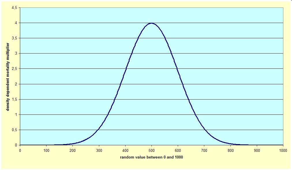
Indeed, density alone is not responsible for density dependent mortality (or self-thinning), and the actual rate varies from case to case and is due to many factors. In predictions, it is impossible to reflect this variation, but can be modelled by randomly changing the rate so that the average of the random rates is equal to the long term average. The distribution of these random rates are modelled as a normal one. Therefore in the second step, if the user decides so, the long-term average density dependent mortality rate is multiplied by a multiplier with an average over many cases of 1 and a normal distribution (see graph).

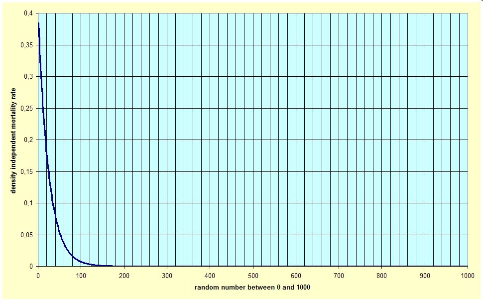
Density independent mortality is modelled by using an exponential function, which is the mortality rate over a scale of random numbers from one to 1000 (see graph). The software generates a random number for each year of the scenario, which is then used to get the mortality rate from the function. This function is taken as a distribution of mortality events, where the smallest, most frequent (>85% of all cases) density independent mortality rate approaches zero, and the highest, once-in-one-thousand-years occurring density independent mortality rate approaches 0,4, which is equivalent to a strong thinning. The density dependent mortality rate is over 0,1 in only 80 of 1000 cases, over 0,2 in only 19 of 1000 cases etc., so the chance of having a large mortality in the max. 50 years of scenario period is pretty low, which is a conservative estimate of extreme events. Thus, the modelling of this density independent mortality due to extreme events is rather for the sake of theoretically complete modelling.

The density independent mortality is only applied in the model if the user selects this option at the beginning of the simulation.

The actual density independent mortality rate over the scenario period for each run can be looked at by selecting the approppriate graph while running the software.

Total mortality rate is taken as the sum of density dependent and density independent mortality rates. It cannot be higher than 0,4 for any year so that cumulative mortality between two consecutive thinnings is very rarely more than what silvicultural practice requires. This total mortality rate is multiplied in any year with the biomass of the previous year to arrive at the mortality estimate.

As it is pointed out above, modelling mortality is theoretically well-based, but is very difficult to model in practice because of the inherent undefineable chain of events that usually results in mortality. Mortality is usually small in well-managed forests that are going to be established for carbon fixation, thus, uncertainty in estimating mortality has a little bearing on the uncertainty at the system level. Yet, efforts were made to model all the important types of mortality because of the well-known nature of mortality, and because of the objective to model the functioning of the forestry system as correctly as possible.

The data for the averages of density dependent mortality in the function of density and site class are good expert estimates. The approximation of the annual variation of the density dependent mortality intensity is purely based on theoretical assumptions without any data. The same is true for density independent mortality, where the distirbution is an educated guess approximation of what may be the case in reality.

Because no predictions can be made for the future, random values are used to generate random patterns. Because of this, separate runs of the same scenario definition (that is, when all assumptions and input data are the same) may result in different values with respect to the distribution of carbon between the various pools, as well as the overall carbon content of the system.

Thinnings are forestry operations when selected trees are cut. The aim of cutting trees can be either silvicultural, when the better growth of the remaining trees is aimed at, or timber harvest, or both. In all cases, the amount of biomass decreases, and the pools of dead wood and, sometimes, the wood products increases.

Thinning has been an essential part of the forestry operations in Hungary, and is expected to remain so, although the timing and intensity of the cuttings may change over time.

The timing and the amount of thinnings have for decades been well defined in the Hungarian forestry practice. The principle is that thinnings must be made before mortality ensues, and the intensity of thinnings ensures economic feasibility of the operations. It is supposed that those and only those trees are cut during thinnings in practice that are really necessary to be cut.

Thinning regime, i.e. the timing and intensity of cuttings, depends on species and site (yield class). The regime is defined by intensity factors by age and yield class for each species. These factors are the ratio of the volume of wood cut (i.e. "thinning") and the stock volume with the typical value being around 0.2-0,3. The factors were calculated from data of the latest yield tables for the respective species. These tables not only contain data for growth, but also for thinning. However, these tables only give data for five year periods. In practice, however, thinnings are not necessarily made in five year periods, rather at lags of a few years to 30 years. The lag, i.e. the time between two consecutive thinnings, was determined by modifying the published data in the so called "silvicultural models" for these species (Solymos 1984). These models recommend when thinnings are to be done, and what the remaining stand should look like (in terms of stand characteristics like number of stems and basal area). It was necessary to modify the timing of thinnings, because these models were created before 1980, and silvicultural practice has changed in two respects since then. Firstly, the lags are longer, since thinnings cost too much, and second, the rotation age has been increased, especially on poor sites, again because of economic considerations.

The thinning factors are calculated for the length of the lag from the annual potential thinning volumes, contained in the yield table, by summing them up as potential thinning volume between two thinnings. The factors are parts of the knowledge base of the model, that is, they are the results of long term silvicultural research, and are incorporated in the files that are used during running. Although the system was not designed to enable the user to change them, it is possible to make changes to both timing and intensity. The user can check the thinning regime by clicking on the approppriate button while running the software.

As it is described in the mortality section above, it is assumed in the silvicultural models that no mortality occurs because of the careful thinnings. However, forestry practice is suboptimal, and mortality occurs. Therefore, not all trees can be cut at the thinnings (in year t) that are suggested by the intensity factors. Because mortality can occure in several years before the cutting of trees, the mortality of these years before thinning or final cutting must be summed up for maximum five years (denoted by sum(M) below) and deducted from the cut (T_s) that would otherwise be made according to the normal practice silvicultural system ("s" in the index of notations below). Thus, if the total mortality is greater than zero, realized thinning (T_t) (and likewise final cutting) is decrased by the amount of mortality:

Thinning intensity factors are long-term averages by species and yield classes. At any specific stand, the factor may vary due to local conditions, change of the silvicultural philosophy, economic situation of the forestry company and others. It is impossible to model all possible cases, and the user must able to judge to what extent the silviculture of the modelled forest follows the "silvicultural models" that are used in CASMOFOR. Indeed, the effect of thinning intensity is that carbon moves from one pool to another within the whole forestry system, and as long as one is interested in the amount of carbon fixed in the whole system, it does not make a big difference in which pool carbon is fixed.

Please also note that the thinning intensity factors themselves are calculated from volumes, but are in fact applied to aboveground tree biomass values. The effect of this is similar to the above.

Final cutting is the last event of the timber production, and it ends the life of the mature trees of the forest. All trees of a stand are cut at final cutting, thus the pool of biomass of trees on the cleared land becomes zero after final cutting.

It is assumed that the forest that went through final cutting is reforested or regenerated the year after the final cutting. It is also assumed that the same species are used before and after the final cutting, and the final cutting does not harm site, i.e., the yield class of the stand remains the same.

Final cutting is modelled just like thinning. The only difference is, of course, that whereas only a part of the trees are cut during thinnings, all trees are cut at final cutting, so the thinning intensity factor is equal to 1 if there is no mortality.

Similarly to thinning, mortality (sum(M), see at thinning) may occur befor final cutting, and can decrease the amount of final cutting (FC_st). However, only mortality in the year ("t" in the index in the function) of final cutting can decrease the amount of final cutting that would occur if there were no mortality ("s" in the index in the function below):

The timings of final cutting by species and yield class are part of the knowledge base of the model, that is, they are the results of long term silvicultural research, and are incorporated in the files that are used during running. The system was not designed to enable the user to change them, and the maximum rotation age is 120 years. The user can check the rotation ages by clicking on the approppriate button while running the software.

The rotation ages were taken from yield tables and so called silvicultural models. They are ages when mean annual increment have reached their maximum, ensuring optimal rotation length for timber production.

Final cutting as a process can be modelled very precisely. The only problematic issue may be the timing. However, rotation ages were selected so that no pests, pathogens or other agents can cause damage to the stand, so, under normal conditions, no loss of carbon in the system due to inapproppriate selection of the rotation age is assumed (and, of course, no extra carbon can be fixed either by using different rotation ages).

The fate of wood after harvesting (either in thinnings or final cuttings) depends on market and economic situations, the transportation infrastructure within the forests (logging roads, forest roads) and outside the forests (highways etc.) and others. Eventually, some timber is left in the forest, some of it is processed and transported as fuelwood, and some as commercial timber. In both moving and processing wood and timber, machines are used in modern forestry, which involves carbon dioxide emission.

Transportation, at this stage of modelling, is modelled by applying a universal emission factor for each ton of wood that is supposed to be moved from the forest. Wood processing is similarly simply modelled by using a ratio that is the fraction of wood to be processed that becomes fuelwood.

Transportation and wood processing are complicated processes that depend very much on local conditions. These include distance from the forest to the wood processing mill and marketing places, transportation infrastructure (roads and trucks etc.), processing machines and technology, final wood products etc. It is impossible in a prediction to account for all these factors, only average values can be used. It must also be noted that, for decades until trees grow large, these processes do not considerable affect the overall carbon fixation of afforestation projects.

Decomposition is the breaking down of dead organic matter (whether in forest or as wood products) due to the activity of various organisms, and physical processes. During this process, most organic compounds break down to more sipmle compounds, and , eventually, to carbon dioxide, which gets back to the air. Some organic compounds cannot be broken down, or only very very slowly, thus some carbon practically stays out of the carbon cycle.

Note that, in CASMOFOR, decomposition of dead organic matter within the soil (i.e. soil respiration) is not modelled, so decomposition only means the break-down of any organic matter (wood, bark and branches, leaves, roots) that becomes dead due to any reason (thinning or mortality), or of any wood product that is not burnt.

Decomposition is only modelled in a simple way. No practical data are available on the various complicated processes that result in the release of carbon dioxide from the dead organic matter. Decomposition is taken as a simple linear process, and constants are used that are equal to the time (in years) that elapses until all breakable compounds are broken down. (The rate of unbrokeable compounds is also set, using IPCC defaults, and are modelled here for good measure only. In the long term, these compounds increase soil carbon content. This increase is, this way, a function of the rate of dead organic matter production, and, ultimately, a function of carbon assimilation by plants.)

The amount of carbon released to the air is thus calculated by the following formula:

R_t is the amount of carbon released (in other words, the amount of carbon that decreases the amount of carbon fixed in the system),

br is the rate of breakable organic compounds relative to all organic compounds (= 1 - ubr, which is the rate of unbreakable organic compounds).

While br values used here are identical for all dead organic matter pools (dead wood, dead roots, dead leaves), dr values are different, because the speed of decomposition of these pools are considerably different. For example, firewood is usually burnt within one year after harvesting, whereas dead root parts may remain in the soil for decades. Therefore, the above formula is used for each dead organic matter pools with respective dr values.

However important it is in the biochemical cycles, decomposition belongs to the less known processes in the forests. We do not have good data that could be used for the modelling purposes in CASMOFOR. Therefore, the simple modelling approach described above is only a first order approximation of what happens with carbon after the trees and their parts die. Not even uncertainty estimates can be provided. The rates used are from the literature, and they are uniformely used accross species, sites, age, size and other characteristics of forests and wood products that may substantially modify the actual rates. Modelling decomposition is applied in CASMOFOR for good measure only, and uncertainty is high with respect to the fate of carbon in dead organic matter.

Soil carbon may change due to conversion, or may be affected by disturbance due to forestry operations. Converting an area to forest may result in increasing soil carbon in case a cropland is converted, but it may result in a temporary loss of carbon in case grassland is converted.

Forestrz operations include soil preparation and final harvest. When soil is prepared for sowing or planting, it may be disturbed e.g. by ploughing, whereas it may be disturbed by the wheels of big machines or trunks of big trees when final harvest is being done. When soil is disturbed, its organic particles, which can mainly be found in the uppermost layears which are subjects to disturbances, get in contact with the air and are emitted to the air mainly in the form of CO₂. It is suggested that by far the most emissions take place due to forestations.

The increase of the organic content is modelled so that a certain small portion of the dead organic matter from leaves, branches, wood and roots remains in the soil pool. After some years, this increase is offset by soil respiration, however, it is assumed that this respiration is small compared to the input in the first 75 years (see graph a. below). Thus, soil respiration is modelled to be so for 75 years that the net carbon stock changes of the soils are due to the transfer of dead organic matter from the other pools to the soil minus soil respiration. (Therefore, the factor in the knowledge base to account for the "ratio of dead organic matter that does not decompose, but increases soil organic matter content" is, in fact, a net value of this factor and the factor that should be used for soil respiration). 75 years after the afforestation, soil respiration is assumed to be equal to the input, i.e. no more carbon is added to the soil.

On converted cropland, only this increase is modelled (see graph a. below). On converted grassland, there is a loss that is modelled by the difference between the gains in graph a. below and the loss in graph b. below up to 75 years after conversion. Both the graphs below, as well as the equations based on them are taken from Horvath et al. (2006).

The effects of disturbances are due to human interventions that are not whithin the boundaries of CASMOFOR, and they are very difficult to model. Therefore, no modelling has been attempted. However, the user may study the effects of these disturbances by setting a simple value when running the model. This value will be used for all species, for all yield classes, and for all forestations. The emissions due to final harvests are included in emissions due to forestations. No emissions linked to thinnings are included.

Carbon loss due to afforestation is also modelled using pre-defined values in user.xls, which can be changed by the user if the loss from soil modelled by an approppriate soil model or measured at specific sites is known (it is assumed that it does not vary much even if the user runs different afforestation scenarios).

The accounting for net removals due to conversion, and emissions due to human induced disturbances are highly uncertain, and no estimate exists concerning this uncertainty.

Burning is quickly transforming dead organic matter, wood in first place, into carbon dioxide, energy and ash. Burning is the main process when utilizing fuelwood, but some dead organic matter is burnt in forests, too.

The burning of fuelwood happens in the year following the one in which fuelwood is produced (in thinnings and final cuttings). The burning of most of the fuelwood results in carbon-dioxide emission, however, a certain amount remains in the system with ash.

With respect to the burning of woody debris in the forest after thinnings, the same values are used as in the greenhouse gas emission report of the country to the UNFCCC.

The transformation of carbon of the fuelwood into released carbon is a straightforward process. However, it may happen in reality that not all firewood is burnt in one year, or some wood is also burnt that were produced in earlier years. In the long run, however, these fluctuations extinguish each other, and the error of estimating carbon release through burning remains very small.

Concerning the size of the small fracton of the carbon that stays unreleased with ash, the IPCC default value is used. The uncertainty of the estimate of this fraction remains unknown.

Fossil fuel is burnt in machines even in forestry. Forestry activities involve the use of various types of machines in all types of forestry operations from soil preparation to thinnings and final cuts. These machines are run on gasoline, and emit carbon into the air. The modelling of the forestry system therefore must include this emission, too. Without estimating this emission it would not be possible to see whether forestry is a net emitter or net remover.

It must be noted that burning of wood entails that fossil fuel of the same energy content is not burnt. Since wood is renewable, but fossil fuel is not, burning of wood and fixing the emitted carbon again decreases, on the long run, the carbon emitted through human activity.

Similarly to many processes, fossil fuel burning can only be modelled by applying average values. These are estimated values per ha of afforestations and per cubic meter wood cut. (Data are from Marosvölgyi B., West-Hungarian University, personal communication.)

Quite naturally, the accuracy of this emission is low due to the highly variable local conditions. However, it can be stated that the energy usage, and the carbon emission, of the forestry operations is low compared to the energy and carbon fixed by the forests. Since the primary objective of CASMOFOR is to see how much is the net carbon fixation of the forests, the accuracy of modelling this emission is acceptable.

All wood products have their life cycle. This is highly variable, since there are many types of wood products: it can be very short for paper and very long for structural wood in constructions. Yet, after short or long life, these wood products are not used, and are either recycled, or burnt, or deposited where they decompose.

Due to the highly variable life cycles, it is very difficult to model even average life cycles. It not only depends on the wood product, but it rapidly changes in our era due to the changing needs and technologies. Only rough average expert judgements are used in CASMOFOR to account for the length of the life cycle.

Expert judgements are only used to estimate average life cycle lengths. This means that the actual value can be twice as much or only half. However, when focusing on the basic aim of the model to estimate carbon fixation of the whole forestry system, the uncertainty associated with the estimation of lifetime of wood products only plays a minor role for decades, and it can become important only decades after the wood was cut, which itself happens decades after afforestation.

Age (yr)	Yield class
Age (yr)	1	2	3	4	5	6
5	(yield data)	(yield data)	(yield data)	(yield data)	(yield data)	(yield data)
10	(yield data)	(yield data)	(yield data)	(yield data)	(yield data)	(yield data)
15	(yield data)	(yield data)	(yield data)	(yield data)	(yield data)	(yield data)
20	(yield data)	(yield data)	(yield data)	(yield data)	(yield data)	(yield data)
25	(yield data)	(yield data)	(yield data)	(yield data)	(yield data)	(yield data)
...	...	...	...	...	...	...
120	(yield data)	(yield data)	(yield data)	(yield data)	(yield data)	(yield data)

Yield class	Species
Yield class	one species, constant area increase	one species, varying annual area increase	constant ratio of several species	varying ratio of several species
one yield class	--	Table 2	--	Table 3
constant ratio of maximum six yield classes	--	Table 4	--	Table 5
varying ratio of maximum six yield classes	Table 4	Table 4	Table 5	Table 5